Consider a continuous time Markov process \(X_t\) on the time interval \([0,T]\) and with value in the state space \(\mathcal{X}\). This defines a probability \(\mathbb{P}\) on the set of \(\mathcal{X}\)-valued paths. Now, it is often the case that one has to consider a perturbed, also sometimes called “twisted”, probability distribution \(\mathbb{Q}\) defined as
\[ \frac{d\mathbb{Q}}{d\mathbb{P}}(x_{[0,T]}) = \frac{1}{\mathcal{Z}} \, \exp[g(X_T)] \tag{1}\]
for a normalization constant \(\mathcal{Z}\) and some function \(g: \mathcal{X}\to \mathbb{R}\). For example, collecting a noisy observation \(y_T \sim \mathcal{F}(X_T) + \textrm{(noise)}\) at time \(T\), the distribution \(\mathbb{Q}\) defined with the log-likelihood function \(g(x) = \log \mathbb{P}(y_T \mid X_T=x)\) describes the dynamics of the Markov process \(X_t\) conditioned on the observation \(y_T\); we will use this interpretation in the following since this is the most common use case and gives the most intuitive interpretation. With this interpretation, it is clear that the normalization constant \(\mathcal{Z}\) is the model evidence \(\mathbb{P}(y_T)\) and that the initial distribution of the conditioned process \(\mathbb{Q}(x_0)\) is the conditional law \(X_0 \mid y_T\) and is given by \(\mathbb{P}(x_0) \, \mathbb{P}(y_T \mid x_0) / \mathbb{P}(y_T)\). Doob h-transforms are a powerful tool to describe the dynamics of the conditioned process.
For convenience, let us use the notation \(\mathbb{E}_x[\ldots] \equiv \mathbb{E}[\ldots \mid x_t=x]\). For a test function \(\varphi: \mathcal{X}\to \mathbb{R}\) and a time increment \(\delta > 0\), we have
\[ \begin{align*} \mathbb{E}[\varphi(x_{t+\delta}) | x_t, y_T] &= \mathbb{E}_{x_t}[\varphi(x_{t+\delta}) \, \exp(g(x_T)) ] \, / \, \mathbb{E}_{x_t}[\exp(g(x_T))]\\ &= \frac{ \mathbb{E}_{x_t}[\varphi(x_{t+\delta}) \, h(t+\delta, x_{t+\delta})] }{h(t, x)}. \end{align*} \tag{2}\]
We have introduced the important function \(h:[0,T] \times \mathcal{X}\to \mathbb{R}\) defined as
\[ h(t, x) \; = \; \mathbb{E} {\left[ \exp[g(x_T)] \mid x_t = x \right]} \; = \; \mathbb{P}(y_T \mid x_t = x). \]
One can readily check that the function \(h\) satisfies the Kolmogorov equation
\[ (\partial_t + \mathcal{L}) \, h = 0 \]
with boundary condition \(h(T,x) = \exp[g(x)]\). Furthermore, denoting by \(\mathcal{L}\) the infinitesimal generator of the Markov process \(X_t\), we have:
\[ \begin{align*} \mathbb{E}_{x_t}[\varphi(x_{t+\delta}) & h(t+\delta, x_{t+\delta}) ] \; = \; \varphi(x_t) h(t, x_t) \\ &+ \; \delta \, (\partial_t + \mathcal{L})[h \, \varphi] \, (t, x_t) \; + \; o(\delta). \end{align*} \tag{3}\]
The infinitesimal generator \(\mathcal{L}^{\star}\) of the conditioned process is
\[ \mathcal{L}^{\star} \varphi(t, x_t) = \lim_{\delta \to 0^+} \; \frac{\mathbb{E}[\varphi(x_{t+\delta}) | x_t, y_T] - \varphi(x_t)}{\delta}. \]
Plugging Equation 3 within Equation 2 directly gives that
\[ \mathcal{L}^{\star} \varphi \; = \; \frac{(\partial_t + \mathcal{L})[h \, \varphi]}{h} \; = \; \frac{\mathcal{L}[\varphi\, h]}{h} + \varphi\frac{\partial_t h}{h}. \]
Some details:
\[ \begin{align*} \mathbb{E}[\varphi(x_{t+\delta}) | x_t, y_T] &= \frac{ \mathbb{E}_{x_t}[\varphi(x_{t+\delta}) \, h(t+\delta, x_{t+\delta})] }{h(t, x)}\\ &= \frac{ \varphi(x_t) h(t, x_t) + \delta (\partial_t + \mathcal{L})[h \, \varphi] \, (t, x_t)}{h(t, x_t)} + o(\delta)\\ &= \varphi(x_t) + \delta \, \frac{(\partial_t + \mathcal{L})[h \, \varphi] \, (t, x_t)}{h(t, x_t)} + o(\delta). \end{align*} \] Since \(\varphi\) does not depend on time, we have \((\partial_t + \mathcal{L})[h \, \varphi] = \varphi\, \partial_t h + \mathcal{L}[h \, \varphi]\) and this gives the announced result.
The generator \(\mathcal{L}^{\star}\) describes the dynamics of the conditioned process. In fact, the same computation holds with a more general change of measure of the type \[ \textcolor{green}{\frac{d\mathbb{Q}}{d\mathbb{P}}(x_{[0,T]}) = \frac{1}{\mathcal{Z}} \, \exp {\left\{ \int_{0}^T f(s, X_s) \, ds + g(x_T) \right\}} } \tag{4}\]
for some function \(f:[0,T] \times \mathcal{X}\to \mathbb{R}\). One can define the function \(h\) similarly as
\[ \textcolor{green}{ h(t, x_t) \; = \; \mathbb{E} {\left[ \exp {\left\{ \int_{t}^T f(X_s) \, ds + g(x_T) \right\}} \mid x_t \right]} }. \tag{5}\]
This function satisfies the Feynman-Kac formula \((\partial_t + \mathcal{L}+ f) \, h = 0\) and one obtains entirely similarly that the probability distribution \(\mathbb{Q}\) describes a Markov process with infinitesimal generator
\[ \textcolor{green}{\mathcal{L}^{\star} \varphi \; = \; \frac{(\partial_t + \mathcal{L}+ f)[h \, \varphi]}{h} \; = \; \frac{\mathcal{L}[h \, \varphi]}{h} + {\left( \frac{\partial_t h} {h} + f \right)} \, \varphi.} \tag{6}\]
Some details:
An interpretation of the conditioned process is as follows. Suppose for example that every \(\delta\) units of time, one observes a noisy measurement \(y_t\) of the state \(x_t\) with log-likelihood \(f(t, x_t) \, \delta\), as well as a final observation at time \(T\) with log-likelihood \(g(x_T)\). For example, this could be a stream of noisy measurements with Gaussian noise of variance proportional to \(1/\delta\) concluded at time \(T\) with a final measurement; in other words, one very frequently observes the state with very noisy measurements and finally makes a more precise observation at time \(T\). In the regime \(\delta \to 0\), the log-likelihood of that stream \(y_{0:T}\) of observations is precisely: \[ \int_0^T f(s, X_s) \, ds + g(X_T). \] Conditioning on these frequent observations then leads to the change of measure in Equation 4. The computations of the conditioned generator then follow similarly as before. We have: \[ \begin{align*} \mathbb{E}[\varphi(x_{t+\delta}) | x_t, y_{0:T}] &= \mathbb{E}[\varphi(x_{t+\delta}) | x_t, y_{t:T}]\\ &= \frac{ \mathbb{E}_{x_t}[\varphi(x_{t+\delta}) \, \exp {\left\{ \int_{t}^T f(s, X_s) \, ds + g(x_T) \right\}} ] }{h(t, x)} \end{align*} \] where \(h\) is defined in Equation 5. The rest of the computation follows similarly as before. First, express \(\exp {\left\{ \int_{t}^T f(s, X_s) \, ds + g(x_T) \right\}} \) as \[ \exp {\left\{ \int_{t}^{t+\delta} f(s, X_s) \, ds \right\}} \, \exp {\left\{ \int_{t+\delta}^T f(s, X_s) \, ds + g(x_T) \right\}} , \] and write that \(\exp {\left\{ \int_{t}^{t+\delta} f(s, X_s) \, ds \right\}} = 1 + f(t, x_t) \, \delta + o(\delta)\) for small \(\delta\). Then conditioned on \(x_{t+\delta}\) to obtain: \[ \begin{align*} \mathbb{E}[\varphi(x_{t+\delta}) | x_t, y_{t:T}] &= \frac{ \mathbb{E}_{x_t}[\varphi(x_{t+\delta}) \, (1 + f(t, x_t) \, \delta) \, h(t+\delta, x_{t+\delta})] }{h(t, x)} + o(\delta)\\ &= \frac{ \mathbb{E}_{x_t}[\varphi(x_{t+\delta}) \, h(t+\delta, x_{t+\delta})] }{h(t, x)} + \delta \, \varphi(x_t) \, f(t, x_t) + o(\delta). \end{align*} \] The rest of the computations are then identical to before.
To see how this works, let us see a few examples:
General diffusions
Consider a diffusion process
\[ dX = b(X) \, dt + \sigma(X) \, dW \]
with generator \(\mathcal{L}\varphi= b \nabla \varphi+ \tfrac12 \, \sigma \sigma^\top : \nabla^2 \varphi\) and initial distribution \(\mu_0(dx)\). We are interested in describing the dynamics of the “conditioned” process given by the probability distribution \(\mathbb{Q}\) defined in Equation 4. Algebra applied to Equation 6 then shows that
\[ \mathcal{L}^\star \varphi\; = \; \mathcal{L}\varphi+ \underbrace{\frac{\varphi\, (\partial_t + \mathcal{L}+ f)[h]}{h}}_{=0} + \sigma \, \sigma^\top \, (\nabla \log h) \, \nabla \varphi \]
where the function \(h\) is described in Equation 5. Since \((\partial_t + \mathcal{L}+ f) \, h = 0\), this reveals that the probability distribution \(\mathbb{Q}\) describes a diffusion process \(X^\star\) with dynamics
\[ dX^\star = b(X^\star) \, dt + \sigma(X^\star) \, {\left\{ dW + \textcolor{blue}{u^\star(t, X^\star)} \, dt \right\}} . \]
The additional drift term \(\sigma(X^\star) \, \textcolor{blue}{u^\star(t, X^\star)} \, dt\) is involves a “control” \( \textcolor{blue}{u^\star(t, X^\star)}\) with \[ \textcolor{blue}{u^\star(t, x) = \sigma^\top(x) \, \nabla \log h(t, x)}. \tag{7}\]
Note that the initial distribution of the conditioned process is
\[ \mu_0^\star(dx) = \frac{1}{\mathcal{Z}} \, \mu_0(dx) \, h(0,x). \]
Unfortunately, apart from a few straightforward cases such as a Brownian motion or an Ornstein-Uhlenbeck process, the function \(h\) is generally intractable. However, there are indeed several numerical methods available to approximate it effectively.
Brownian bridge
What about a Brownian motion in \(\mathbb{R}^D\) conditioned to hit the state \(x_\star \in \mathbb{R}^D\) at time \(t=T\), i.e. a Brownian bridge? In that case, the function \(h\) is given by
\[ h(t,x) = \mathbb{P}(B_T = x_\star \mid B_t = x) = \exp {\left\{ -\frac{\|x-x_\star\|^2}{2 \, (T-t)} \right\}} / \mathcal{Z}_{T-t} \]
for some irrelevant normalization constant \(\mathcal{Z}_{T-t}\) that only depends on \(T-t\). Plugging this into Equation 7 gives that the conditioned Brownian \(X^{\star}\) motion has dynamics
\[ dX^\star \;=\; \textcolor{blue}{- \frac{X^\star - x_\star}{T-t} \, dt} + dB. \]
The additional drift term \(-(X^\star - x_\star)/(T-t)\) is intuitive: it points in the direction of \(x^\star\) and gets increasingly large as \(t \to T\).
Positive Brownian motion
What about a scalar Brownian conditioned to stay positive at all times? Let us consider \(T\) and let us condition first on the event that the Brownian motion stays positive within \([0,T]\) and later consider the limit \(T \to \infty\). The function \(h\) reads
\[ h(t,x) = \mathbb{P} {\left( \text{$B_t$ stays $>0$ on $[t,T]$} \mid B_t=x \right)} . \]
This can easily be calculated with the reflection principle. It equals
\[ h(t,x) = 1 - 2 \, \mathbb{P}(B_T < 0 \mid B_T = x) = \mathbb{P}(\sqrt{T-t} \, \| \xi \| < x) \]
for a standard Gaussian \(\xi \sim \mathcal{N}(0,1)\). Plugging this into Equation 7 gives that the additional drift term is
\[ \nabla \log h(t,x) = \frac{\exp {\left( -x^2 / (2 \, (T-t)) \right)} }{x} \quad \to \quad \frac{1}{x} \]
as \(T \to \infty\). This shows that a Brownian motion conditioned to stay positive at all times has a upward drift of size \(1/x\),
\[ dX^\star \;=\; \frac{1}{X^{\star}} + dB. \]
Incidentally, it is the dynamics of a Bessel process of dimension \(d=3\), i.e. the law of the modulus of a three-dimensional Brownian motion. More generally, if one conditions a Brownian motion to stay within a closed domain \(\mathcal{D}\), the conditioned dynamics exhibit a repulsive drift term of size about \(1/\textrm{dist}(x, \partial \mathcal{D})\) near the boundary \(\partial \mathcal{D}\) of the domain, as described below.
Brownian motion staying in a domain
What about a Brownian motion conditioned to stay within a domain \(\mathcal{D}\) forever? As before, consider an time horizon \(T\) and define the function \(h\) as
\[ h(t,x) = \mathbb{P} {\left( \text{$B_t$ stays in $\mathcal{D}$ on $[t,T]$} \mid B_t=x \right)} . \]
One can see that the function \(h\) satisfies the PDE
\[ (\partial_t + \Delta) \, h = 0 \]
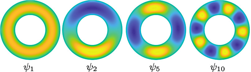
and equals zero on the boundary \(\partial \mathcal{D}\) of the domain. Furthermore \(h(t,x) \to 1\) as \(t \to T\) for all \(x \in \mathcal{D}\). Consider the eigenfunctions \(\psi_k\) of the negative Laplacian \(-\Delta\) with Dirichlet boundary conditions on \(\partial \mathcal{D}\). Recall that \(-\Delta\) is a positive operator with a discrete spectrum \(\lambda_1 \leq \lambda_2 \leq \ldots\) of non-negative eigenvalues. The eigenfunction corresponding to the smallest eigenvalue \(\lambda_1\) is the principal eigenfunction \(\psi_1\) and it is standard that it is a positive function within the domain \(\mathcal{D}\), as a “slight” generalization of the Perron-Frobenius in linear algebra shows it. Expanding \(h\) in the basis of eigenfunctions \(\psi_k\) gives that
\[ h(t,x) = \underbrace{c_1 \, e^{-\lambda_1 \, (T-t)} \, \psi_1(x)}_{\textrm{dominant contribution}} + \sum_{k \geq 2} c_k \, e^{-\lambda_k \, (T-t)} \, \psi_k(x). \]
Since we are interested in the regime \(T \to \infty\), it holds that
\[ \nabla_x \log h(t,x) \; \to \; \nabla \log \psi_1(x).\]
This shows that the conditioned Brownian motion has a drift term expressed in terms of the principal eigenfunction \(\psi_1\) of the Laplacian:
\[ dX^\star \;=\; \textcolor{blue}{ \nabla \log \psi_1(X^\star) \, dt} + dB. \]
For example, if \(\mathcal{D}\equiv [0,L]\) for a 1D Brownian motion, the principal eigenfunction is \(\psi_1(x) = \sin(\pi \, x /L)\). This shows that there is a upward drift of size \(\sim 1/x\) near \(x \approx 0\) and a downward drift of size \(\sim 1/(L-x)\) near \(x \approx L\).