
These notes are a brief introduction to Lagrange multipliers and convex duality, with as little technical detail as possible since the epsilon-delta proofs can be found in many places. Consider the problem of minimizing a smooth function \(f:\mathbb{R}^d \to \mathbb{R}\). In the absence of constraints, the first-order condition is of course
\[ \nabla f(x_\star)=0. \]
Indeed, if the gradient is non-zero, one can move a little in the direction \(-\nabla f\) and decrease the function. In some sense, a lot of these notes are about generalizing this simple remark to the case of equality and inequality constraints. Constraints only change one thing: some directions are no longer available, which indeed means that the condition \(\nabla f(x_\star)=0\) will need to be relaxed in different ways. As we will see, the notion of Lagrange multipliers and Lagrange duality are the natural generalizations of this simple idea.
Equality constraints
Suppose first that the feasible set is described by \(r\geq1\) smooth equality constraints,
\[ h_1(x)=0, \quad h_2(x)=0, \quad \ldots, \quad h_r(x)=0 \]
for scalar-valued functions \(h_a:\mathbb{R}^d\to\mathbb{R}\). Near a feasible point where the gradients \(\nabla h_a\) are linearly independent, this is a smooth surface of dimension \(d-r\). At a local minimum \(x_\star\), the directional derivative of \(f\) vanishes along every tangent vector, so \(\nabla f(x_\star)\) is orthogonal to the tangent space. Since that tangent space is the orthogonal complement of the span of the constraint gradients, there exist multipliers \(\nu_a\in\mathbb{R}\) such that
\[ \textcolor{green}{ \nabla f(x_\star) + \sum_{a=1}^r \nu_a\,\nabla h_a(x_\star) =0.} \tag{1}\]
At an optimum, the objective gradient has no tangent component.
Inequality constraints
Consider \(m\geq1\) smooth inequality constraints
\[ g_1(x)\leq0, \quad g_2(x)\leq0, \quad \ldots, \quad g_m(x)\leq0 \]
for scalar-valued functions \(g_i:\mathbb{R}^d\to\mathbb{R}\). At a feasible point \(x_\star\), let \(\mathcal{A}(x_\star)=\{i:g_i(x_\star)=0\}\) be the set of active constraints. Under the regularity conditions discussed below, the tangent cone is the intersection of the half-spaces
\[ \left< \nabla g_i(x_\star),v \right>\leq0, \qquad i\in\mathcal{A}(x_\star). \]
If equality constraints \(h_a(x)=0\) are also present, we additionally require \(\left< \nabla h_a(x_\star),v \right>=0\). At a local minimum, \(\left< \nabla f(x_\star),v \right>\geq0\) for every vector in this cone. By Farkas’ lemma, this is equivalent to
\[ \nabla f(x_\star) +\sum_{a=1}^r\nu_a\,\nabla h_a(x_\star) +\sum_{i\in\mathcal{A}(x_\star)}\lambda_i\,\nabla g_i(x_\star)=0, \]
with \(\nu_a\in\mathbb{R}\) and \( \textcolor{green}{\lambda_i\geq 0}\). In general, \(-\nabla g_i(x_\star)\) need not be a feasible direction: it may violate another active constraint. The sign restriction on the multipliers comes from the whole cone of feasible directions.
Setting \(\lambda_i=0\) for inactive constraints lets us write the sum over all constraints:
\[ \textcolor{green}{ \nabla f(x_\star) +\sum_{a=1}^r\nu_a\,\nabla h_a(x_\star) +\sum_{i=1}^m\lambda_i\,\nabla g_i(x_\star)=0.} \tag{2}\]
The condition that inactive constraints have zero multipliers is called complementary slackness:
\[ \textcolor{green}{\lambda_i\,g_i(x_\star)=0.} \tag{3}\]
Either the constraint \(g_i\) has some slack, in which case its multiplier \(\lambda_i\) vanishes, or the multiplier is nonzero, in which case the constraint is active.
The Lagrangian
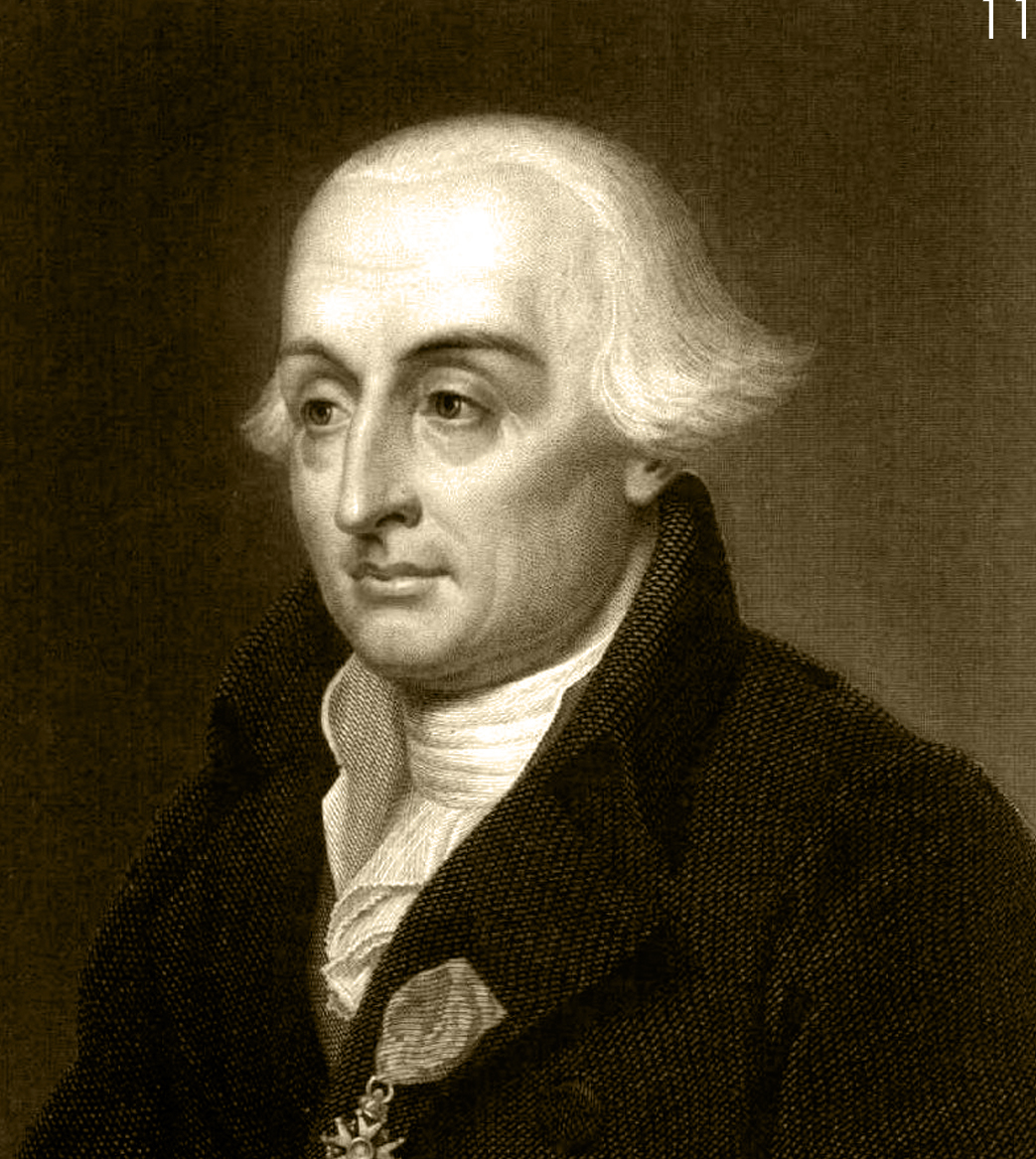
The Lagrangian collects the objective and constraints:
\[ \mathcal{L}(x,\lambda,\nu) = f(x) + \sum_{i=1}^m \lambda_i g_i(x) + \sum_{a=1}^r \nu_a h_a(x). \]
The stationarity condition Equation 2 is \(\nabla_x\mathcal{L}(x_\star,\lambda,\nu)=0\). Together with feasibility and complementary slackness, it gives the Karush–Kuhn–Tucker (KKT) conditions:
\[ \textcolor{green}{ \begin{aligned} \nabla_x\mathcal{L}(x_\star,\lambda,\nu)&=0,\\ g_i(x_\star)&\leq 0, & h_a(x_\star)&=0,\\ \lambda_i&\geq 0, & \lambda_i g_i(x_\star)&=0. \end{aligned} } \tag{4}\]
At a regular local minimum, these conditions are necessary. For a general nonconvex problem, they do not guarantee local or global optimality.
A small pathology
The arguments above identify the tangent cone with the directions satisfying the linearized constraints. This identification can fail. Consider minimizing \(f(x)=x\) subject to \(g(x)=x^2\leq0\). The feasible set is \(\{0\}\), so \(x_\star=0\) is the global minimum, but stationarity would require
\[ 0=\nabla f(0)+\lambda\nabla g(0)=1+\lambda\cdot0, \]
which is impossible. The constraint gradient vanishes, so the linearized inequality allows every direction, whereas the tangent cone is \(\{0\}\).
Constraint qualifications rule out this degeneracy and ensure that KKT conditions are necessary at a local minimum. One sufficient condition is the linear independence constraint qualification (LICQ): the gradients of all equality constraints and active inequality constraints are linearly independent. For affine constraints, the linearization is exact, so KKT necessity holds even when these gradients are linearly dependent.
The convex case
In the unconstrained case, a stationary point of a convex function is a global minimum. For the constrained analogue, let \(A\in\mathbb{R}^{r\times d}\) and \(b\in\mathbb{R}^r\), and consider the convex program:
\[ \begin{aligned} \textrm{minimize} \qquad & f(x),\\ \textrm{subject to} \qquad & g_i(x)\leq 0,\\ & Ax=b, \end{aligned} \tag{5}\]
where \(f\) and the functions \(g_i\) are convex. With affine equalities \(Ax=b\), the feasible set is convex. The Lagrangian is also convex in \(x\) for any \(\lambda\geq0\) and \(\nu\):
\[ \mathcal{L}(x,\lambda,\nu) = f(x)+\sum_i \lambda_i g_i(x)+\nu^\top(Ax-b). \]
Now, assume that a feasible point \(x_\star\) and multipliers \((\lambda_\star,\nu_\star)\) satisfy the KKT conditions Equation 4. Since the Lagrangian is convex in \(x\), stationarity \(\nabla_x \mathcal{L}(x_\star,\lambda_\star,\nu_\star) = 0\) implies that the function \(x \mapsto \mathcal{L}(x,\lambda_\star,\nu_\star)\) has a global minimum at \(x_\star\):
\[ \mathcal{L}(x_\star,\lambda_\star,\nu_\star) \leq \mathcal{L}(x,\lambda_\star,\nu_\star) \]
for every \(x\). Furthermore, \(f(x_\star) = \mathcal{L}(x_\star,\lambda_\star,\nu_\star)\) by complementary slackness and feasibility. For any feasible \(x\), we also have \(\mathcal{L}(x,\lambda_\star,\nu_\star) \leq f(x)\) since \(\lambda_\star \geq 0\) and \(g_i(x)\leq 0\). Combining these two inequalities gives:
\[ \textcolor{green}{f(x_\star) = \mathcal{L}(x_\star,\lambda_\star,\nu_\star) \leq \mathcal{L}(x,\lambda_\star,\nu_\star) \leq f(x)} \]
for every feasible \(x\). Thus, in a convex problem, the KKT conditions are sufficient for global optimality:
\[ \textcolor{green}{\textrm{KKT} \quad \Longrightarrow \quad \textrm{global optimum}.} \tag{6}\]
No constraint qualification is needed for this direction.
For KKT conditions to be necessary, a constraint qualification is still needed, as the example \(x^2\leq0\) shows. For a convex problem, Slater’s condition requires a point \(\bar x\) satisfying the equalities and strictly satisfying every inequality:
\[ \textcolor{blue}{ \textrm{Slater:} \qquad \qquad A\bar x=b \quad \text{and} \quad g_i(\bar x)<0 \; \text{for all } \; 1 \leq i \leq m. } \]
The condition is named after Morton Slater, whose Lagrange Multipliers Revisited is available in the Cowles Foundation archive. He is distinct from John Slater, of Slater determinant fame in quantum mechanics. Under Slater’s condition, an optimal point admits KKT multipliers. Combining this with Equation 6 gives
\[ \textcolor{green}{ \textrm{global optimum} \quad \Longleftrightarrow \quad \textrm{KKT}.} \tag{7}\]
Convexity makes KKT sufficient; the constraint qualification makes KKT necessary.
The dual problem
The discussion above hints at a more general principle. For multipliers \(\lambda \geq 0\) and arbitrary \(\nu\), the dual function is defined as the infimum of the Lagrangian over \(x\):
\[ q(\lambda,\nu) = \inf_x \mathcal{L}(x,\lambda,\nu). \]
For any feasible \(x\) and \(\lambda\geq0\), we have \(\mathcal{L}(x,\lambda,\nu)\leq f(x)\). Consequently,
\[ q(\lambda,\nu) \leq f(x) \]
for every feasible \(x\), without any convexity assumption. Taking the infimum over feasible \(x\) gives
\[ \textcolor{green}{q(\lambda,\nu) \leq p_\star} \]
where \(p_\star\) is the primal optimal value. Maximizing this lower bound gives the dual problem:
\[ \sup_{\lambda\geq 0,\,\nu} q(\lambda,\nu) = \textcolor{green}{d_\star \; \leq \; p_\star} = \inf_{x \text{ feasible}} f(x) \]
This is weak duality, and it does not require convexity. For the convex program above, Slater’s condition gives (Boyd and Vandenberghe 2004, chap. 5)
\[ \textcolor{green}{d_\star=p_\star.} \tag{8}\]
This is strong duality. When the primal value is finite, Slater’s condition also ensures that the dual optimum is attained.
Proof
Assume \(p_\star\) is finite and discard redundant equality constraints, so that \(A\) has full row rank. Consider the set \(\mathcal C\) of all \((u,v,t)\in\mathbb{R}^m\times\mathbb{R}^r\times\mathbb{R}\) such that, for some \(x\),
\[ g_i(x)\leq u_i, \qquad Ax-b=v, \qquad f(x)\leq t. \]
This set is convex, and \((0,0,p_\star)\) is a boundary point, even if the primal infimum is not attained. A supporting hyperplane therefore gives a nonzero normal \((\lambda,\nu,\mu)\) with
\[ \lambda^\top u+\nu^\top v+\mu t\geq\mu p_\star \qquad\text{for every }(u,v,t)\in\mathcal C. \]
Since \(\mathcal C\) is closed under increasing \(u\) or \(t\), we have \(\lambda\geq0\) and \(\mu\geq0\). Suppose \(\mu=0\). Substituting a Slater point gives
\[ \lambda^\top g(\bar x)\geq0. \]
Because every \(g_i(\bar x)<0\), this forces \(\lambda=0\). The supporting inequality then becomes \(\nu^\top(Ax-b)\geq0\) for every \(x\). This implies \(A^\top\nu=0\), hence \(\nu=0\) because \(A\) has full row rank, contradicting the nonzero normal.
Thus \(\mu>0\), and we can normalize it to \(1\). Substituting \((u,v,t)=(g(x),Ax-b,f(x))\) gives
\[ f(x)+\lambda^\top g(x)+\nu^\top(Ax-b)\geq p_\star \qquad\text{for every }x. \]
Taking the infimum over \(x\) gives \(q(\lambda,\nu)\geq p_\star\). Weak duality supplies the reverse inequality, so \(d_\star=q(\lambda,\nu)=p_\star\).
Saddle point interpretation
Suppose strong duality holds, \(p_\star=d_\star\), and both the primal and dual optima are attained at \(x_\star\) and \((\lambda_\star,\nu_\star)\). By the definition of \(q\) and primal feasibility,
\[ p_\star =q(\lambda_\star,\nu_\star) \leq\mathcal{L}(x_\star,\lambda_\star,\nu_\star) \leq f(x_\star) =p_\star. \]
All inequalities are therefore equalities: \(x_\star\) minimizes \(\mathcal{L}(\cdot,\lambda_\star,\nu_\star)\), and complementary slackness holds. For any dual-feasible \((\lambda,\nu)\), primal feasibility also gives \(\mathcal{L}(x_\star,\lambda,\nu)\leq f(x_\star)\). Together these yield the saddle-point property
\[ \textcolor{green}{ \mathcal{L}(x_\star,\lambda,\nu) \leq\mathcal{L}(x_\star,\lambda_\star,\nu_\star) \leq\mathcal{L}(x,\lambda_\star,\nu_\star) } \]
for every \(x\) and every \(\lambda\geq0\), \(\nu\in\mathbb{R}^r\). This saddle-point formulation motivates a number of primal-dual algorithms for convex optimization.