Reversing a diffusion

Imagine a scalar diffusion process \(\{X_t\}_{t=0}^T\) defined on the interval \([0,T]\),
\[dX = \mu(X) \, dt + \sigma \, dW\]
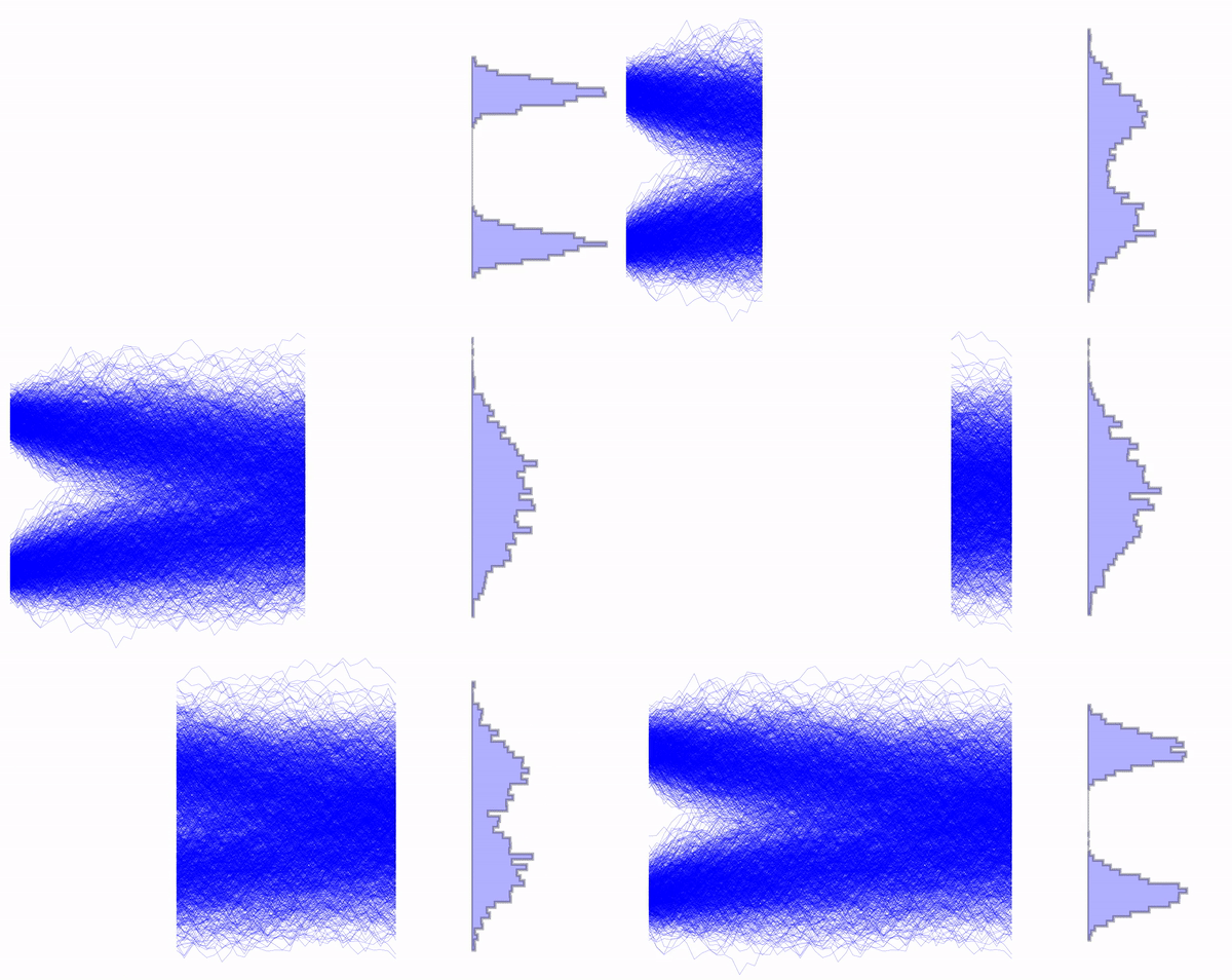
where \(\mu(X)\) is the drift term, \(\sigma\) is the diffusion coefficient, and \(dW\) is a Wiener process. Denote the distribution of this process at time \(t\) (\(0 \leq t \leq T\)) as \(p_t(dx)\) with an initial distribution of \(p_0(dx)\). Now, what happens if we reverse time and examine the process backward? In other words, consider the time-reversed process \(\overleftarrow{X}\) defined as
\[\overleftarrow{X}_s = X_{T-s}.\]
Intuitively, the process \(\overleftarrow{X}\) is also a diffusion on the interval \([0, T]\), but with an initial distribution \(\overleftarrow{X}_0 \sim p_T(dx)\). To gain intuition, consider an Euler discretization of the forward process:
\[X_{t+\delta} = X_{t} + \mu(X_t)\, \delta + \sigma \, \sqrt{\delta} \, \mathbf{n} \tag{1}\]
where \(\mathbf{n}\sim \mathcal{N}(0,1)\) represents a noise term independent from \(X_{t}\), and \(\delta \ll 1\) is a time increment. Re-arranging terms and making the approximation \(\mu(X_t) \approx \mu(X_{t+\delta})\) gives that
\[X_{t} \approx X_{t+\delta} - \mu(X_{t+\delta})\, \delta + \sigma \, \sqrt{\delta} \, (-\mathbf{n}). \tag{2}\]
This seems to suggest that the time-reversed process follows the dynamics \(d\overleftarrow{X} = -\mu(\overleftarrow{X}) \, dt + \sigma \, dW\) started from \(\overleftarrow{X}_0 \sim p_T(dx)\). However, this conclusion is incorrect because this would suggest that the time-reversed of a standard Brownian motion (where \(\mu(x) \equiv 0\)) starting at zero is also a Brownian motion starting at \(p_T(dx) = \mathcal{N}(0,T)\), which is clearly not the case. The flaw in this argument lies in assuming that the noise term \(Z\) is independent of \(X_{t+\delta}\), which is not true, rendering the Euler discretization argument invalid.
Deriving the dynamics of the backward process in a rigorous manner is not straightforward (Anderson 1982) (Haussmann and Pardoux 1986). What follows is a heuristic derivation that proceeds by estimating the mean and variance of \(X_{t}\) given \(X_{t+\delta} = x_{t+\delta}\), assuming \(\delta \ll 1\). Here, \(x_{t+\delta}\) is treated as a fixed and constant value, and we are only interested in the conditional distribution of \(X_t\) given \(x_{t+\delta}\). Bayes’ law gives
\[\mathbb{P}(X_t \in dx | x_{t+\delta}) \propto p_t(x) \, \exp\left\{ -\frac{\left( x_{t+\delta} - [x + \mu(x) \, \delta] \right)^2}{2 \sigma^2 \, \delta} \right\},\]
where the exponential term corresponds to the transition of the forward diffusion for \(\delta \ll 1\). Using the 1st order approximation
\[p_t(x) \approx p_t(x_{t+\delta}) \,\exp\left( \langle \nabla \log p_t(x_{t+\delta}), (x-x_{t+\delta})\rangle\right),\]
eliminating multiplicative constants and higher-order error terms, we obtain:
\[\mathbb{P}(X_t \in dx | x_{t+\delta}) \propto \exp\left\{ -\frac{\left( x - [x_{t+\delta} - \mu(x_{t+\delta}) \delta + {\color{red} \sigma^2 \, \nabla \log p_t(x_{t+\delta}) \, \delta} ] \right)^2}{2 \sigma^2 \, \delta} \right\}.\]
For \(\delta \ll 1\), this is transition of the reverse diffusion
\[ d\overleftarrow{X}_t = \textcolor{red}{-}\mu(\overleftarrow{X}_t) \, dt \; + {\color{red} \sigma^2 \, \nabla \log p_{T-t}(\overleftarrow{X}_t) \, dt} \; + \; \sigma \, dB. \tag{3}\]
The notation \(B\) is used to emphasize that this Brownian motion is distinct from the one used in the forward diffusion. The additional drift term, denoted as \({\color{red} \sigma^2 \, \nabla \log p_t(\overleftarrow{X})}\), is intuitive: it pushes the reverse diffusion toward regions where the forward diffusion spent a significant amount of time, i.e., where \(p_t(dx)\) is large. Note the minus sign in front of the original drift term \(\mu(X) \, dt\) It interesting to note that if \(X\) is a Langevin diffusion reversible with respect to a probability density \(\pi(x)\),
\[ dX = \tfrac{\sigma^2}{2} \nabla \log \pi(X) \, dt + \sigma \, dB, \]
then the reverse diffusion diffusion Equation 3 reads simply as
\[ d\overleftarrow{X}_t = \tfrac{\sigma^2}{2} \nabla \log \pi(\overleftarrow{X}_t) \, dt \; + {\color{red} \sigma^2 \, \nabla \log [p_{T-t} / \pi](\overleftarrow{X}_t) \, dt} \; + \; \sigma \, dB. \]
Note that there is no minus sign in front of the original drift term. This highlight that, when at stationarity, the reverse diffusion indeed follows the same dynamics as the forward diffusion. More generally, consider a bridging sequence of distributions \(\pi_t(dx)\) indexed by time parameter \(t \in [0,T]\). If one can find a control function \(c_t(x)\) such that the controlled Langevin diffusion
\[ dX_t = \tfrac{\sigma^2}{2} \, \nabla \log \pi_t(X_t) \, dt \textcolor{blue}{+ c_t(X_t)} \, dt + \sigma \, dB, \]
is such that \(X_t \sim \pi_t(dx)\) for all time \(0 \leq t \leq T\), then the reverse diffusion reads is
\[ d\overleftarrow{X}_t = \tfrac{\sigma^2}{2} \, \nabla \log \pi_{T-t}(\overleftarrow{X}_t) \, dt \textcolor{red}{- c_{T-t}(\overleftarrow{X}_t)} \, dt + \sigma \, dB. \]
A discussion on how his relates to a generalizations of the Crooks fluctuation theorem can be found in this other note. The popular “denoising diffusion models” (Ho, Jain, and Abbeel 2020) can be seen as discretizations of the backward process Equation 3, employing various techniques to estimate the additional drift term from data.
Denoising Score Matching & Tweedie formula
The previous section shows that a quantity often referred to as the “score” in machine learning (ML) literature, i.e. \(\mathcal{S}_t(x) \equiv \nabla_x \log p_t(x)\), naturally arises when a diffusion process runs backward in time. Interestingly, it is worth noting that since the beginning of times statisticians have been using the term “score” to refer to the other derivative, i.e. the derivative with respect to a model’s parameter, which is a completely different object!
Consider a Brownian diffusion process \(dX = \sigma \, dW\) initiated from a distribution \(p_0(dx)\). If this process is ran forward for a duration \(\delta>0\), we have:
\[X_{\delta} = X_0 + \mathcal{N}(0, \sigma^2 \, \delta)\]
where \(X_0 \sim p_0(dx)\). Now, focusing on a specific sample \(y = X_{\delta}\), the backward dynamics \(d\overleftarrow{X} = \sigma^2 \, \nabla \log p_t(\overleftarrow{X}) \, dt + \sigma \, dB\) suggests that for sufficiently small \(\delta\), the following approximation holds:
\[ \mathbb{E}[X_0 \, | X_{\delta} = y] \; { \color{\red} \approx} \; y + \nabla \log p_{\delta}(y) \, \sigma^2 \delta. \tag{4}\]
Maybe surprisingly, in the case of Brownian dynamics (no drift), this relationship holds exactly, even for arbitrarily large time increments \(\delta>0\). This observation attributed in (Efron 2011) to Maurice Tweedie (1919–1996) has a straightforward proof. Specifically, if \(X \sim p_0(dx)\), then \(Y = X + \mathcal{N}(0, \Gamma^2)\) has a density given by:
\[ p_Y(dy) = \int p_0(x) \, \rho_{\Gamma}(y-x) \, dx \]
where \(\rho_{\Gamma}(z) \propto \exp[-z^2/(2 \Gamma^2)]\) is a centred Gaussian with variance \(\Gamma^2\). It follows that
\[ \frac{ \mathbb{E}[X \, | Y = y]-y}{\Gamma^2} = \frac{ \int \left( \frac {x-y }{\Gamma^2} \right)\, p_0(x) \, \rho_{\Gamma}(y-x) \, dx }{\int p_0(x) \, \rho_{\Gamma}(y-x) \, dx}. \]
Since \(\nabla_y \log \rho_{\Gamma}(y-x) = (x-y)/\Gamma^2\), this also read:
\[ \frac{ \mathbb{E}[X \, | Y = y]-y}{\Gamma^2} = \nabla_y \log \left\{ \int p_0(x) \, \rho_{\Gamma}(y-x) \, dx \right\}. \]
This leads to Tweedie’s formula:
\[ \mathbb{E}[X \, | Y = y] \; {\color{red} =} \; y + \Gamma^2 \, \nabla \log p_Y(y), \]
which is exactly the same as Equation 4 but with an equality sign: no approximation needed! Interestingly, this is what Machine-Learners often refer to as “denoising score matching” (Vincent 2011): if we have access to a large number of samples \((X_i,Y_i)\), where \(X_i \sim p_0(dx)\) and \(Y_i = X_i + \mathcal{N}(0, \Gamma^2)\), and fit a regression model \(F_{\theta}\) by minimizing the mean-squared error \(\theta \mapsto \mathbb{E} \|X - F_{\theta}(Y)\|^2\), then Tweedie formula shows that in the limit of infinite samples and with sufficient flexibility in the regression model \(F_{\theta_\star}(y) = y + \Gamma^2 \nabla \log p_Y(y)\). This allows one to estimate \(\nabla \log p_Y\) from data, which is often a good approximation of \(\nabla \log p_0\) if the variance \(\Gamma^2\) of the added noise is not too large. Indeed, things can go bad if \(\Gamma^2 \ll 1\) and the number of training data is not large enough, no free lunch!
Generalizations of Tweedie’s formula
Tweedie’s formula can be slightly generalized, which can be useful in practice. Suppose one would like to estimate the score \(\nabla_y \log p_Y(y)\) of the marginal distribution \(p_y(y) = \int_{\mathcal{X}} p_{(X,Y)}(x,y) \, dx\). Since \(\mathbb{E}[\nabla_y \log p_{X|Y}(X) | Y=y] = 0\), we have that
\[ \begin{align*} \nabla_y \log p_Y(y) &= \nabla_y \log p_Y(y) + \mathbb{E}[\nabla_y \log p_{X|Y}(X \mid y) | Y=y] \\ &= \mathbb{E}[\nabla_y \log p_{(X,Y)}(X,Y) | Y=y]\\ &= \mathbb{E}[\nabla_y \log [p_{X}(X) \, p_{Y|X}(Y|X)] | Y=y]\\ &= \mathbb{E}[\nabla_y \log p_{Y|X}(Y|X) | Y=y]. \end{align*} \]
This means that if we can simulate from \(X|Y=y\) and evaluate \(\nabla_y \log p_{Y|X}(Y|X)\), then we can estimate \(\nabla_y \log p_Y(y)\) by Monte-Carlo. If one has access to a large number of samples \((X_i,Y_i)\), one can also set up a regression problem as done in the previous section. In the setting when the marginal \(p_X(X)\) is available and \(Y\) is only a small perturbation of \(X\) it may be beneficial to exploit the knowledge of \(p_X(X)\) to reduce the variance of the estimator of \(\nabla_y \log p_Y(y)\). Suppose for example that:
\[ Y = \alpha X + Z \]
for additive noise \(Z \sim p_Z(dz)\) independent of \(X\). Then, (De Bortoli et al. 2024) shows that
\[ \nabla_y \log p_Y(y) = \alpha^{-1} \, \times \, \mathbb{E}[\nabla_x \log p_X(X) | Y=y]. \]
In the Gaussian case \(p_Z \sim \mathcal{N}(0, \sigma^2)\), the AR(1) model \(X \mapsto \alpha X + Z\) is reversible with respect to the distribution \(\rho \equiv \mathcal{N}(0, \sigma^2/(1-\alpha^2))\). If one defines \(\widetilde{p}_X(x) = p_X(x)/\rho(x)\) and \(\widetilde{p}_Y(y) = p_Y(y)/\rho(y)\), then one obtains a slightly different formula:
\[ \nabla_y \log \widetilde{p}_Y(y) = \alpha \, \times \, \mathbb{E}[\nabla_x \log \widetilde{p}_X(X) | Y=y] \]
