Fisher-Rao metric
Suppose we want to define a distance on the space of probability densities on \(\mathbb{R}^d\). A natural but naive approach is to use an \(L^2\)-type distance:
\[ d(\rho_1, \rho_2)^2 = \int_{\mathbb{R}^d} |\rho_1(x) - \rho_2(x)|^2 \, dx, \]
where \(\rho_i\) are densities with respect to the Lebesgue measure. However, this definition has several shortcomings. For instance, if we change the base measure to \(\mu(x) \, dx\) for some positive density \(\mu\), and define the distance as
\[ \int \left|\frac{\rho_1(x)}{\mu(x)} - \frac{\rho_2(x)}{\mu(x)}\right|^2 \mu(x) \, dx, \]
we obtain a different value. Perhaps more troubling, the distance is not invariant under reparametrizations. Let \(T\) be a diffeomorphism of \(\mathbb{R}^d\), and set \(y = T(x)\). Then the transformed densities become \(\rho^Y_i(y) = \rho^X_i(x) \, |J_T(x)|^{-1}\), where \(J_T\) is the Jacobian determinant. In general,
\[ \int |\rho^Y_1(y) - \rho^Y_2(y)|^2 \, dy \neq \int |\rho^X_1(x) - \rho^X_2(x)|^2 \, dx, \]
so the distance depends on the choice of coordinates. That is, measuring in Cartesian or polar coordinates yields different results—an undesirable feature. Ideally, we seek a distance that is invariant under reparametrizations and changes of base measure, such as the total variation distance,
\[ d_{TV}(\rho_1, \rho_2) = \int_{\mathbb{R}^d} |\rho_1(x) - \rho_2(x)| \, dx. \]
One potential drawback of the total variation distance is that it is not differentiable, which can make it difficult to use in optimization problems. An alternative is to consider \(f\)-divergences, defined as
\[ d_f(\rho_1, \rho_2) = \int_{\mathbb{R}^d} f \left( \frac{d\rho_1}{d\rho_2} \right) \rho_2(dx), \]
where \(f\) is a convex function with \(f(1) = 0\). These divergences are differentiable and invariant under reparametrizations and changes of base measure, although they are not symmetric and thus not true distances. Locally, however, all \(f\)-divergences are equivalent, as a second-order Taylor expansion shows:
\[ d_f(\rho + d \rho, \, \rho) = \textrm{(cst)} \times \int \left( \frac{d \rho}{\rho} \right)^2 \, \rho(dx) + o(\|d \rho\|^2). \]
This means that all these divergences describe the same local geometry, defined by the Fisher-Rao information metric. Furthermore, it is relatively straightforward to derive the global geometry induced by the Fisher information metric. Consider the mapping \(\rho \mapsto \sqrt{\rho}\), which maps a density \(\rho\) to an element of the unit sphere \(\mathcal{S}\) of \(L^2(\mathbb{R}^d)\). Since
\[ \| \sqrt{\rho_1} - \sqrt{\rho_2} \|_{L^2}^2 = d_f(\rho_1, \rho_2) \]
for \(f(x) = |1 - \sqrt{x}|^2\), and we have just seen that any \(f\)-divergence is locally equivalent to the Fisher-Rao metric, it follows that the geometry induced by the Fisher-Rao information information metric is the same as the geometry induced by the \(L^2\)-norm on the unit sphere of \(L^2(\mathbb{R}^d)\). This implies that the geodesic distance between two densities \(\rho_1\) and \(\rho_2\) is given (up to an irrelevant constant) by the \(L^2\)-geodesic distance between the points \(\sqrt{\rho_1} \in \mathcal{S}\) and \(\sqrt{\rho_2} \in \mathcal{S}\). In other words, the geodesic distance, i.e. the Fisher-Rao distance, is given by
\[ d_{FR}(\rho_1, \rho_2) = \arccos \left( \langle \sqrt{\rho_1}, \sqrt{\rho_2} \rangle_{L^2} \right). \]
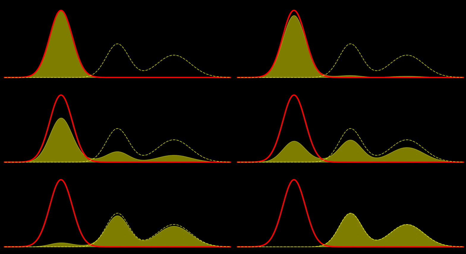
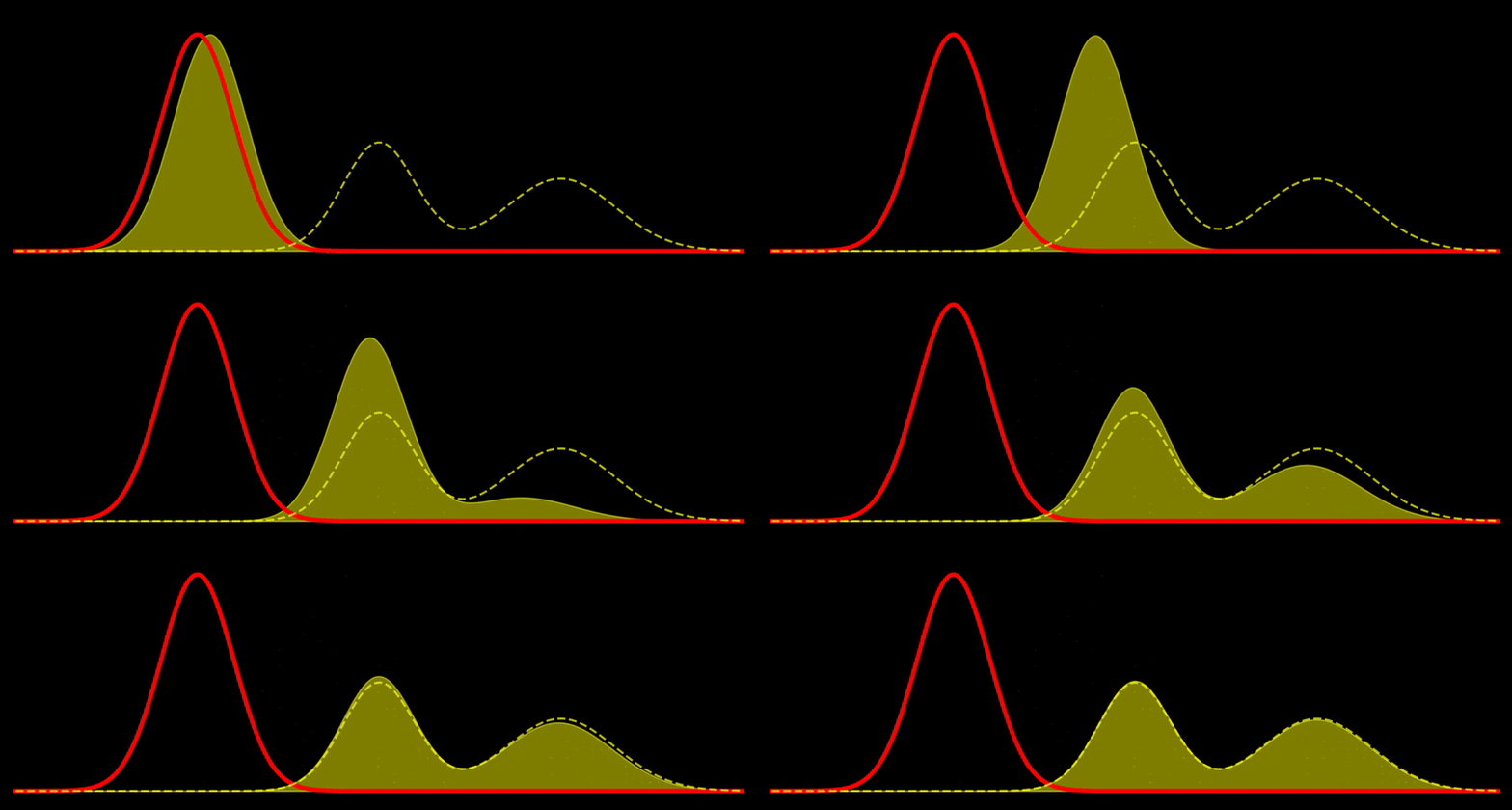
The geodesic path is a great circle, \(t \mapsto \rho_t\), where \(\rho_t \propto \left((1-t) \sqrt{\rho_1} + t \sqrt{\rho_2} \right)^2\) for \(t \in [0,1]\). This shows, for example, that the Fisher-Rao geodesic between two Gaussian densities is composed of densities that are Gaussian mixtures; i.e., the geodesic is not composed of Gaussian densities in general. In other words, probability mass is not transported along the geodesic but reshaped, unlike the Wasserstein metric, which describes transport of probability mass. Note in passing that the Hellinger distance, defined as
\[ d_H(\rho_1, \rho_2)^2 = \int \left( \sqrt{\rho_1(x)} - \sqrt{\rho_2(x)} \right)^2 \, dx, \]
is just just a slightly rescaled version of the Fisher-Rao distance since they are related by a deterministic function, i.e. \(d_H = \sqrt{2(1-\cos(d_{FR}))}\). In this sense, the Hellinger distance is equivalent to the Fisher-Rao distance, and both describe a “correct” way to measure distances between probability densities for many applications.

Gradient flow
What do gradient flows look like in this Fisher-Rao geometry? For example, for a given distribution \(\pi\), the gradient flow of \(\rho \mapsto \mathrm{KL}(\rho, \pi)\) under the Wasserstein metric is given by the transport equation:
\[ \partial_t \rho = -\nabla \cdot \left( \rho \, \nabla \log \frac{\pi}{\rho} \right), \]
which describes the Langevin dynamics of the process \(dX = \nabla \log \pi(X) \, dt + \sqrt{2} \, dB\), as informally described in these notes. So what does the gradient flow of \(\rho \mapsto \mathrm{KL}(\rho, \pi)\) look like in the Fisher-Rao geometry?
To answer this, one can consider the square-root mapping \(\rho \mapsto \sqrt{\rho} \equiv \Phi(\rho) \in \mathcal{S}\), express everything in terms of \(\Phi(\rho)\), compute the \(L^2\)-gradient on the unit sphere \(\mathcal{S}\) (which is straightforward), and finally map back to the density \(\rho\) using the inverse mapping \(\Phi^{-1}\). One readily finds that the gradient flow is described by:
\[ \partial_t \rho = \log \frac{\pi}{\rho} - \mathbb{E}_\rho \left[ \log \frac{\pi}{\rho} \right]. \]
This is quite intuitive: the flow tries to increase \(\rho\) in regions where \(\rho \ll \pi\) and decrease \(\rho\) in regions where \(\rho \gg \pi\). Discretizing this flow can naturally be done using sampling-based methods. If \(\sum_{i=1}^N w_i \, \delta(x_i)\) is a system of \(N\) weighted particles approximating \(\rho\), following the Fisher-Rao gradient flow corresponds to updating the weights as
\[ w_i \mapsto \frac{ w_i \, (\pi(x_i) / \rho(x_i))^{\varepsilon}}{\sum_{j=1}^N w_j \, (\pi(x_j) / \rho(x_j))^{\varepsilon}} \]
for a small \(\varepsilon> 0\) time-step. Indeed, it is because \(\partial_t \rho(x) = v(x)\), where \(\mathbb{E}_{\rho}[v]=0\), can be discretized by updating the weights as \(w_i \mapsto w_i \, \exp[\varepsilon\, v(x_i)] / Z\). This is very much related to the resampling step in sequential Monte Carlo methods, and the recent article (Crucinio and Pathiraja 2025) make these connections explicit.
